Keep the Channel, Change the Filter: A Smarter Way to Fine-Tune AI Models

Table of Links

Abstract and 1. Introduction

2. Preliminary
3. Methods
4. Experiments
5. Related Works
6. Conclusion and References
7. Details of Experiments
8. Additional Experimental Results

3 Methods

In this section, we decompose convolution filters over a small set of filter subspace elements, referred to as fitler atoms. This formulation enables a new model tuning method via filter subspace by solely adjusting filter atoms.

3.1 Formulation of Filter Decomposition

Our approach involves decomposing each convolutional layer F into two standard convolutional layers: a filter atom layer D that models filter subspace[1 , and an atom coefficient layer α with 1 × 1 filters that represent combination rules of filter atoms, as displayed in Figure 2 (a). This formulation is written as

\

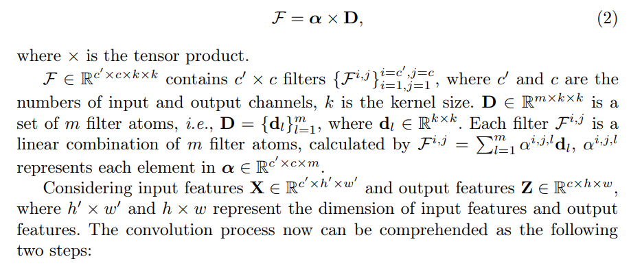
\ • Spatial-only Convolution with D. Each channel of the input features X convolves with each filter atom separately to produce intermediate features

\

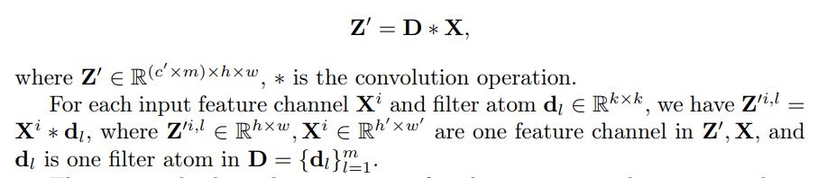
\ This process leads to the generation of m distinct intermediate output channels for each input channel, which is illustrated in Figure 2 (b). In this step, filter atoms focus only on handling the spatial information of input features, and cross-channel mixing is postponed to the next step.

\ • Cross-channel Mixing with α. Subsequently, atom coefficients weigh and linearly combine the intermediate features to produce output features

\ Z = a x Z’

\

\ The spatially invariant channel weights, atom coefficients α, serve as operators for channel mixing, functioning as distinct combination rules that construct the output features from the elemental feature maps generated by the filter atoms. During the model tuning, α is obtained from the pre-trained model and remains unchanged, while only filter atoms D adapt to the target task.

\ Summary. The two-step convolution operation explains different functionalities of filter atoms D and atom coefficients α, which is, D only contribute to spatial convolution and α only perform cross-channel mixing. In practice, the convolution operation is still performed as one layer, without generating intermediate features, to avoid memory cost. In the fine-tuning process, we solely adjust D, which contains a small set of number of parameters, k × k ≪ c′ × c, thereby facilitating parameter-efficient fine-tuning.

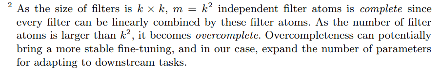
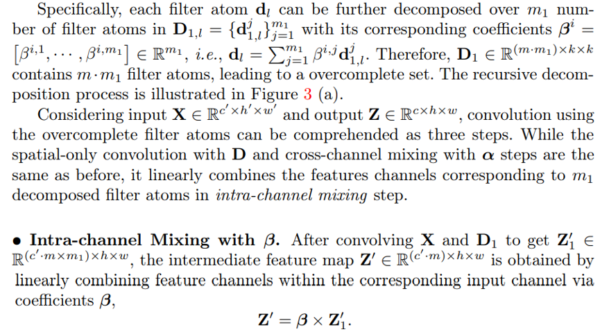
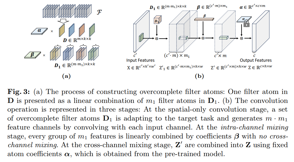
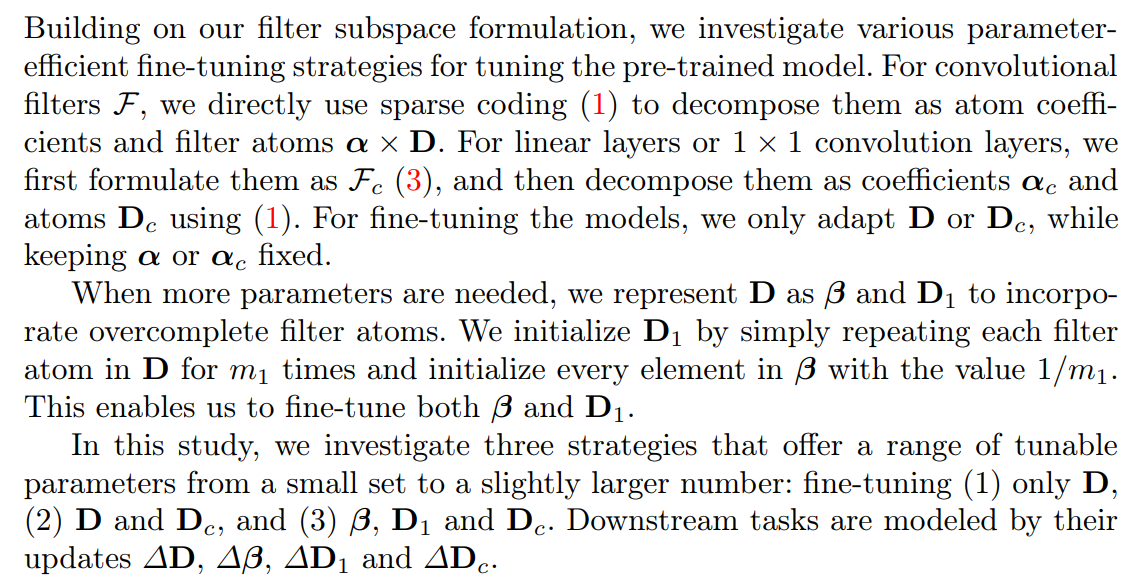
3.2 Overcomplete Filter Atoms

The parameters of filter atoms are extremely small compared with overall model parameters. For instance, the filter atoms constitute a mere 0.004% of the total parameters in ResNet50 [13]. To fully explore the potential of filter subspace fine-tuning, we show next a simple way to construct a set of overcomplete[2] filter atoms by recursively applying the above decomposition to each filter atom, to expand the parameter space for fine-tuning as needed.

\

\

\

3.3 Decomposition of Linear Layers

\

3.4 Parameter Efficient Fine-tuning

\

4 Experiments

In this section, we begin with studying the effectiveness of our method across various configurations to determine the most suitable application scenario for each configuration. Subsequently, we demonstrate that fine-tuning only filter atoms requires far fewer parameters while preserving the capacity of pre-trained models, compared with baseline methods in the contexts of discriminative and generative tasks.

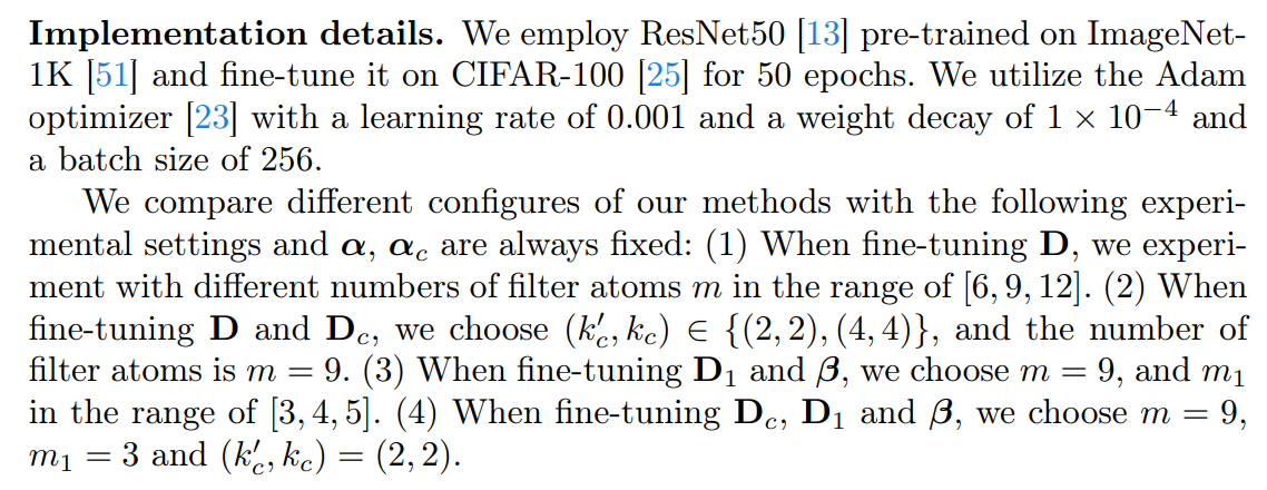
4.1 Experimental Settings

Datasets. Our experimental evaluations are mainly conducted on the Visual Task Adaptation Benchmark (VTAB) [76], which contains 19 distinct visual recognition tasks sourced from 16 datasets. As a subset of VTAB, VTAB-1k comprises a mere 1, 000 labeled training examples in each dataset.

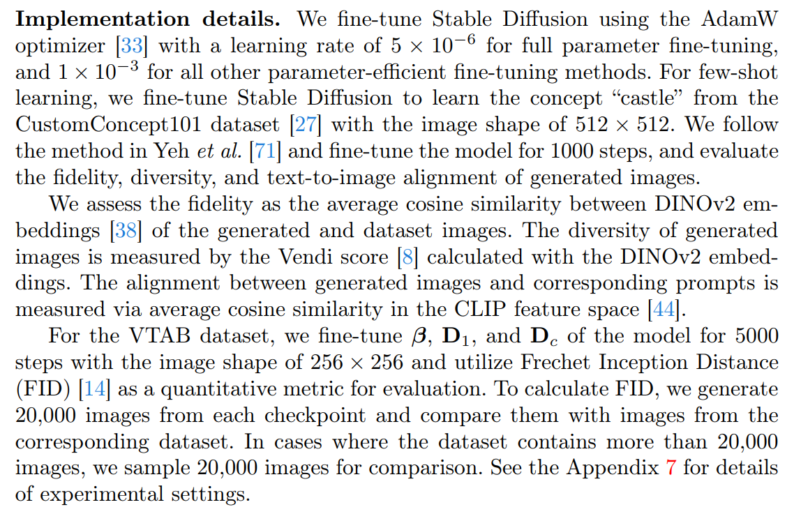
\ Models. For the validation experiment, we choose ResNet50 [13] pre-trained on ImageNet-1K. For discriminative tasks, we choose the convolution-based model, ConvNeXt-B [32] pre-trained on ImageNet-21K as the initialization for finetuning. For generative tasks, we choose Stable Diffusion [49] which contains a downsampling-factor 8 autoencoder with an 860M UNet and CLIP ViT-L/14 as text encoder for the diffusion model. The model is pre-trained on the LAION dataset [54], which contains over 5 billion image-text pairs. More details of pretrained models are listed in the Appendix 7.

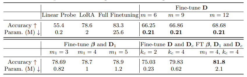
4.2 Validation Experiments

In this section, we study the performance of our approach across various configurations.

\ \

\ \ \

\ \ \

\

4.3 Generative Tasks

In this section, we apply our method to the generative task by evaluating the generative samples from VTAB dataset [76].

\ Baselines. We compare our method to 6 baseline fine-tuning approaches: (i) Full fine-tuning, which entails updating all model parameters during the finetuning process; (ii) LoRA [16], involving the introduction of a low-rank structure of accumulated gradient update by decomposing it as up-projection and downprojection. (iii) LoHa [71] utilizes the Hadamard product across two sets of lowrank decompositions to elevate the rank of the resultant matrix and reduce the approximation error. (iv) LoKr [71] introduces the Kronecker product for matrix decomposition to reduce the tunable parameters. (v) BitFit [74] fine-tunes the bias term of each layer. (vi) DiffFit [69] fine-tunes the bias term, as well as the layer norm and the scale factor of each layer.

\ \

\ \ \

\ \ \ ." />

\ \ \

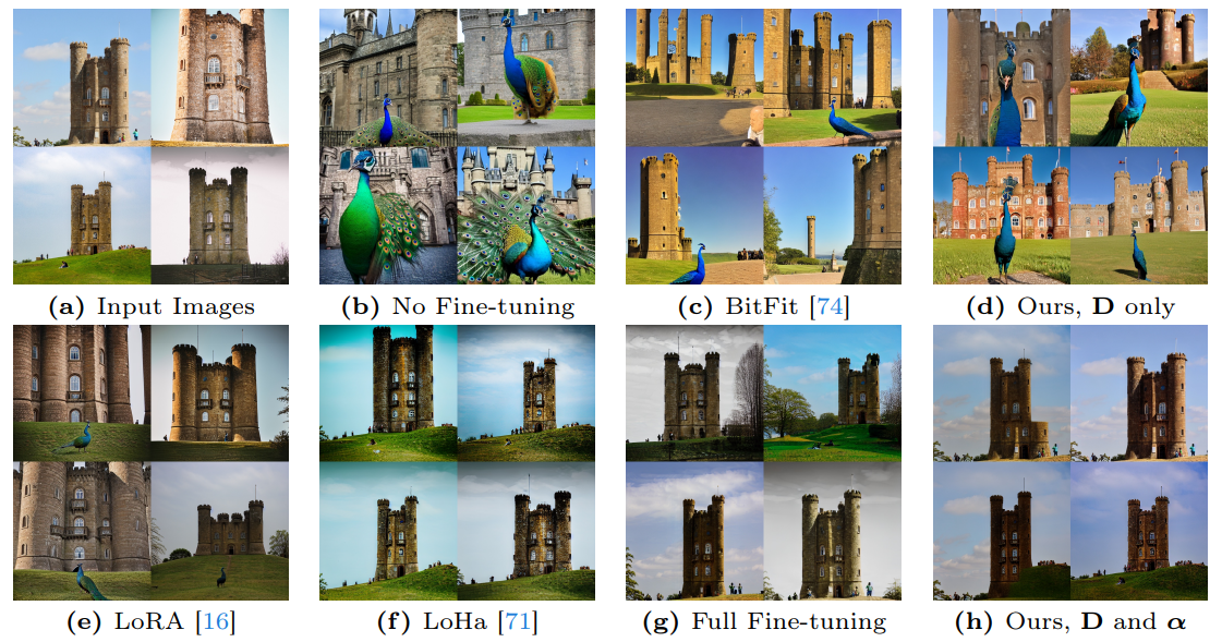
\ \ Methods like LoRA [16] or full fine-tuning potentially update these α, thus, they lead to lower diversity and text-to-image alignment in generated images. In contrast, BitFit [74] and DiffFit [69] mostly fine-tune the bias, leaving α fixed, thus, they have a higher diversity and text-to-image alignment than LoRA. However, they also keep the spatial operation D unchanged, resulting in a lower fidelity score compared with C2. More results can be found in Appendix 8.

\ \

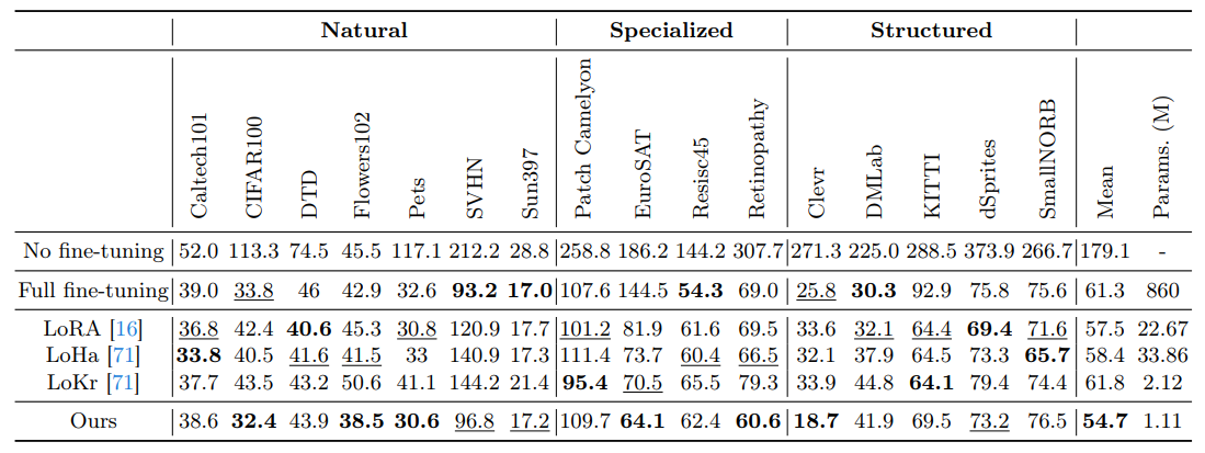
\ \ Performance comparisons on generative transfer learning. We report FIDs of models trained and evaluated on VTAB tasks in Table 3. In contrast to full parameter fine-tuning and LoRA, our approach attains the lowest FID scores (54.7 v.s. 57.5) while employing the least number of fine-tuning parameters (1.11M v.s. 22.67M). Despite fine-tuning only 0.13% of the total model parameters, our method effectively tailors pre-trained Stable Diffusion to align it with the desired target distribution.

4.4 Discriminative Tasks

In this section, we apply our method to the discriminative task, namely the classification on VTAB-1k [76]. We compare our method to 4 baseline fine-tuning approaches: (i) Full fine-tuning, (ii) Linear probing, (iii) BitFit [74], and (iv) LoRA [16].

\ Implementation details. Images are resized to 224 × 224, following the default settings in VTAB [76]. We employ the AdamW [33] optimizer to fine-tune models for 100 epochs. The cosine decay strategy is adopted for the learning rate schedule, and the linear warm-up is used in the first 10 epochs.

\ In this experiment, we fine-tune D and Dc while keeping α and αc fixed, as this configuration delivers adequate accuracy without increasing parameters.

\ Performance comparisons on few-shot transfer learning. We compare the performance of our approach and other baseline methods, and the results

\ \

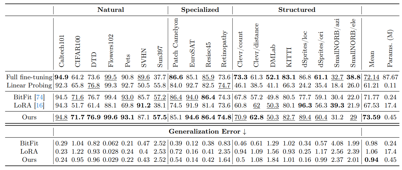
\ \ on VTAB-1k are shown in Table 4. In these tables, the bold font shows the best accuracy of all methods and the underlined font shows the second best accuracy. Our method outperforms other parameter-efficient fine-tuning methods and even outperforms full fine-tuning. Specifically, our method obtains 6% improvement in accuracy compared to LoRA on the VTAB-1k benchmark while utilizing significantly fewer trainable parameters (0.45M v.s. 17.4M).

\ The generalization error is measured by the discrepancy between the training loss and the test loss, with the findings illustrated in Table 4 and Figure 7 from Appendix 8. Our technique, which employs fixed atom coefficients, leads to a comparatively lower generalization error. It means our tuning method better preserves the generalization ability of the pre-trained model.

\

:::info Authors:

(1) Wei Chen, Purdue University, IN, USA ([email protected]);

(2) Zichen Miao, Purdue University, IN, USA ([email protected]);

(3) Qiang Qiu, Purdue University, IN, USA ([email protected]).

:::

:::info This paper is available on arxiv under CC BY 4.0 DEED license.

:::

[1] The filter subspace is a span of m filter atoms D.

\